Tutorial: analyse a set of sessions
This takes a folder of recorded sessions and produces the figures and tables you would look at first. It assumes you have run sessions and know where they were saved.
What you should have
Sessions are saved in a nested structure, and the analysis relies on it:
maze_recordings/
└── grammar/                       <- experiment mode
    ├── habituation/               <- day label
    │   ├── time_2026-05-23_10_00_00mouse6224/
    │   └── time_2026-05-23_10_40_00mouse6225/
    ├── day_1/
    │   ├── time_2026-05-24_09_00_00mouse6224/
    │   └── ...
    └── day_2/
The day label comes from --day on the command line, or the Day label field in the application. If you did not set one, sessions sit directly under the mode folder and the cross-session tools cannot group them by day. That is worth fixing before you collect more.
Step 1: check one session
Start with a single session, because a problem here invalidates everything downstream.
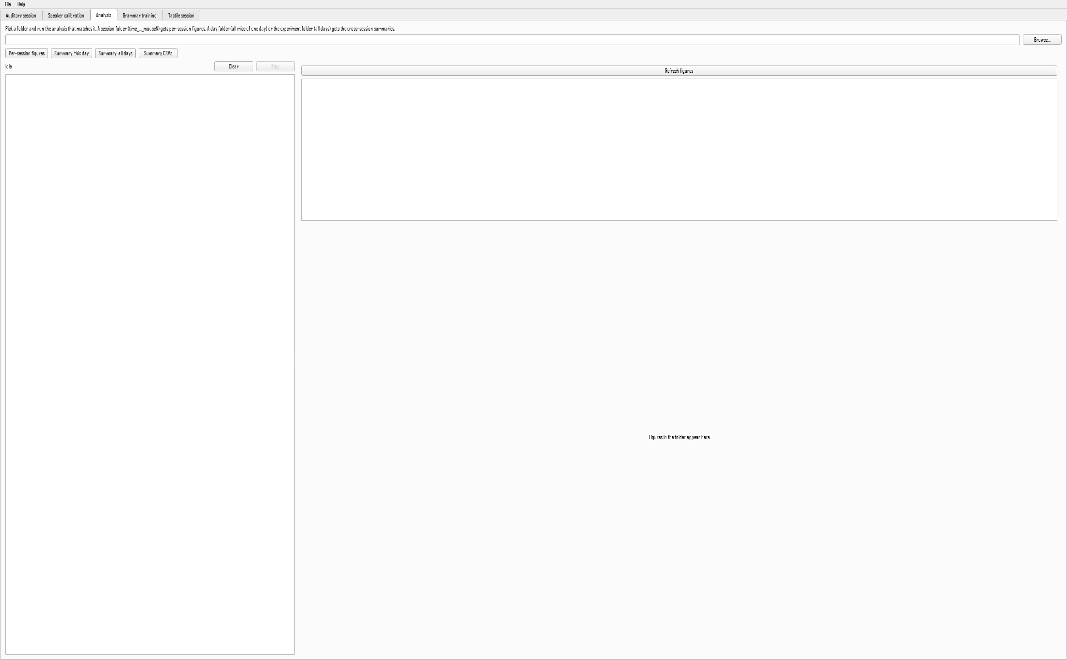
In the application, open the Analysis tab, choose one session folder with Browse, and press Per-session figures. From a terminal:
The figures land in the session folder and are listed in the tab for preview.
What to look for:
- Total time per arm should not be zero for every arm. If it is, detection failed and the session has no usable data.
- Visit counts in the tens to hundreds for an hour-long session. A handful means detection was too strict; thousands means it was too loose and is flickering.
- Time in the maze per block should be a decent fraction of each block. An animal that never entered tells you nothing about the sounds.
Every arm shows zero
The detection baseline was probably measured with something in the maze, or the ROI file no longer matches the camera position. Check session_manifest.json for the settings used, and compare the ROI file against a frame of the video.
Step 2: summarise a day
Once several mice have run on the same day:
or the Summary: this day button. Figures are written into the day folder, one panel per mouse plus a group summary.
The key figure is the preference index per mouse: a value above zero means more time on one category of arm than the other, and the spread across mice tells you whether an effect is consistent or driven by one animal.
Step 3: summarise across days
This adds the cross-day figures: each mouse's trajectory over days, and the group mean. Habituation and silent-baseline sessions are excluded automatically, since they have no sounds to prefer.
Step 4: get the numbers out
Figures are for looking; tables are for statistics.
This writes summary_<day>.csv into each day folder and summary_all_sessions.csv at the root, one row per mouse per day, with time and visit counts per category and the preference index. That file is the starting point for statistics in whatever tool you prefer.
Step 5: the research pipelines
The steps above are the routine ones. For the analyses behind the published work, see the auditory pipeline, which covers the preference index with proper within-trial comparison, mixed-effects models, and the computational model, or the tactile pipeline for choice accuracy and trajectory metrics.
These expect a data root rather than a single session, and several need the [analysis] extra installed:
A checklist before believing a result
- Did detection work in every session, or are some animals represented by a handful of visits?
- Was the speaker calibrated? An uncalibrated speaker makes some frequencies louder, and louder looks like preferred.
- Is the effect present in both counterbalancing groups, where the design has them? An effect that flips with the group is a property of the stimulus, not of the association you meant to test.
- Does the preference survive the arm reshuffle, or is the animal returning to a physical location regardless of what plays there?